GATE Documentation#
GATE is a simulation toolkit for medical imaging and nuclear medicine, and its Monte Carlo engine is based on the popular Geant4 toolkit. This toolkit is developed and maintained by the OpenGATE collaboration, and since Gate10 the macro files have been replaced by python libraries, making it a very user friendly framework to run MonteCarlo simulations.
Although developed primarily for nuclear medicine related Monte Carlo simulations, GATE can also be used HEP simulations. In this page, I have listed a few examples of the use cases in HEP.
Installation and setup#
Below steps are referenced from the OPENGATE documentation page.
First create a python virtual environment to install GATE.
python -m venv GateVenv
source GateVenv/bin/activate
Currently, GATE10 supports python3.11, and not the latest python 3.12. If you’re computer has python3.11, you can create the virtual environment like
python3.11 -m venv GateVenv. This way, inside the virtual environment we will use python3.11Hint
It’s always good to create a virtual environment when you’re installing software that does not use the latest python version or packages, in order to avoid conflicts with dependencies.
Install the python module. Please make sure to include the
-preoption to get the latest release. This will also install all the dependencies needed to run Gate10.pip install --pre opengate
Then you will need to install the Geant4 libraries. For this, simply run the below executable.
opengate_infoThe above executable (and other new executables) will be visible when you’re in the python virtual environment. Also, be patient. It will take some time to download all the Geant4 data.
Once everything is installed, it’s recommend to run some tests by executing,
opengate_testsYou should see almost all the tests will return OK, while some occasional Failed (which is safe to ignore, since some additional packages are not installed yet).
And now you’re all set. Build your own simulations and see how it works 😉
Some additional settings#
Just in case, some additional configuration or packages may be needed if they’re not installed by default. Below are a few of them encountered by me.
Sometimes the there maybe conflicts with the packages versions. For me, it seems numpy 2.0 was installed, and this caused some conflicts when executing
opengate_tests. This can be simply fixed by installing the latest numpy 1.0 version like,python -m pip install numpy==1.26.0
There may be some important packages which are not installed by default, but needed for running simulations. Just install them like
python -m pip install <package-name>pyvista- For visualization of the simulation.
Example 1: Building the ATLAS calorimeter#
Below I list the basic steps in order to create the ATLAS Liquid-Argon (ECal) and Tile (HCal) calorimeters in the barrel section. The complete code can also be viewed from my GitLab page (yet to be uploaded).
Caution
The simulation of the ATLAS calorimeter described below is still very preliminary, and there are a lot aspects which can be improved (and which I hope to improve in the near future). Nevertheless, as you can see from the results (at the very end), this model describes well the particle interaction in the electromagnetic and hadronic calorimeters.
Common definitions#
Below are some common functions and parameters that are useful to make the object definitions simpler.
def createSheet(Object, Size, Trans, Rotate, Material, Color, Mother=""):
    if Mother!="":
        Object.mother = Mother
    Object.size = Size
    if Trans != []:
        Object.translation = Trans
    if Rotate != []:
        rot = Rotation.from_euler('xyz', Rotate, degrees=True)
        Object.rotation = rot.as_matrix()
    Object.material = Material
    Object.color = Color

colors = {"scinti": [0, 0.7, 0.7, 0], "steel": [.9, .9, .9, 0],
          "air": [1, 0, 0, 1], "lead": [.7, .7, .7, 0], "lAr": [0, 1, 1, 1]}

# Define some useful rotations
rot1 = Rotation.from_euler('xyz', [90, 0, 0], degrees=True).as_matrix()
rot2 = Rotation.from_euler('xyz', [45, 0, 0], degrees=True).as_matrix()
Initialization#
First create the GATE simulation, and set the main options
sim = gate.Simulation()

# main options
ui = sim.user_info
ui.g4_verbose = False
ui.g4_verbose_level = 1
ui.visu = visu
ui.visu_type = "vrml"
ui.random_seed = "auto"
ui.number_of_threads = 1
Then import the materials database file.
sim.volume_manager.add_material_database(data_path / "GateMaterials.db")
Create the world we run our simulation
world = sim.world
world.size = [2*m, 2*m, 5*m]
Building the ATLAS electromagnetic calorimeter (ECal)#
After the initialization steps, first lets create the liquid Argon electromagnetic calorimeter.
First create the liquid Argon tank.
argTank = sim.add_volume("Box", "ArgonTank")
createSheet(argTank, [75*cm, 75*cm, 52*cm], [0*cm, 0*cm, 1*m], [], "G4_lAr", colors["lAr"])
Then create the accordion shaped lead sheets, and translate them in the y-axis and z-axis. Note that I chose to create a boolean object combining two simple lead sheets, and duplicate it (but probably there is a smarter way of doing this).
# First make two lead sheets
lead_sheet1 = sim.volume_manager.create_volume("Box", "LeadSheet1")
createSheet(lead_sheet1, [70*cm, 2*mm, 50*mm], [], [], "Lead", colors["lead"], "ArgonTank")
lead_sheet2 = sim.volume_manager.create_volume("Box", "LeadSheet2")
createSheet(lead_sheet2, [70*cm, 2*mm, 50*mm], [], [], "Lead", colors["lead"], "ArgonTank")
# Combine both lead sheets, and make the accordion shape in two steps
lead_wedge1 = unite_volumes(lead_sheet1, lead_sheet2, [0, 24*mm, 24*mm], rot1)
lead_wedge2 = unite_volumes(lead_sheet1, lead_sheet2, [0, 24*mm, 24*mm], rot1)
lead_wedge3 = unite_volumes(lead_wedge1, lead_wedge2, [0, 48*mm, 48*mm], new_name="LeadWedge")

sim.add_volume(lead_wedge3)
lead_wedge3.rotation = rot2
lead_wedge3.translation = gate.geometry.utility.get_grid_repetition([1, 80, 3],[0*mm, 8*mm, 196*mm / np.sqrt(2)])
It should look something like this (minus the particle shower),

Building the ATLAS hadronic tile calorimeter (HCal)#
Then lets create the hadronic tile calorimeter.
First create an air container as a mother object (this is for easy visualization)
# First create an air block as a mother object
air = sim.add_volume("Box", "AirBlock")
createSheet(air, [102*cm, 120*cm, 200*cm], [0*mm, 0*cm, -0.5*m], [], "Air", colors["air"])
Then we create a simple 2x2 definition of the calorimeter cell. Here, we first create the scintillator block, and then place 4 steel sheets inside it.
# Create a small scintillator block
scinti1 = sim.add_volume("Box", "PlasScinti1")
createSheet(scinti1, [17*mm, 40*cm, 40*cm], [], [], "Scinti-C9H10", colors["scinti"], "AirBlock")

# Steel sheet 1
steel_sheet1 = sim.add_volume("Box", "SteelSheet1")
createSheet(steel_sheet1, [14*mm, 20*cm, 20*cm], [-1.5*mm, 10*cm, -10*cm], [], "Steel", colors["steel"], "PlasScinti1")
# Steel sheet 2
steel_sheet2 = sim.add_volume("Box", "SteelSheet2")
createSheet(steel_sheet2, [14*mm, 20*cm, 20*cm], [1.5*mm, 10*cm, 10*cm], [], "Steel", colors["steel"], "PlasScinti1")
# Steel sheet 3
steel_sheet3 = sim.add_volume("Box", "SteelSheet3")
createSheet(steel_sheet3, [14*mm, 20*cm, 20*cm], [-1.5*mm, -10*cm, 10*cm], [], "Steel", colors["steel"], "PlasScinti1")
# Steel sheet 4
steel_sheet4 = sim.add_volume("Box", "SteelSheet4")
createSheet(steel_sheet4, [14*mm, 20*cm, 20*cm], [1.5*mm, -10*cm, -10*cm], [], "Steel", colors["steel"], "PlasScinti1")
Then we replicate the cells into a massive calorimeter block.
scinti1.translation = gate.geometry.utility.get_grid_repetition([60, 3, 5],[17*mm, 40*cm, 40*cm])
It should look something like this (minus the particle shower),

Define the physics and send a particle#
Then we will define the physics as below, and send different particles from the positive Z-direction.
# physics
sim.physics_manager.physics_list_name = "QGSP_BERT_EMV"
sim.physics_manager.set_production_cut("world", "proton", 10 * m)
sim.physics_manager.set_production_cut("world", "electron", 10 * m)
for obj in ["ArgonTank", "LeadWedge", "PlasScinti1", "SteelSheet1", "SteelSheet2", "SteelSheet3", "SteelSheet4"]:
    sim.physics_manager.set_production_cut(obj, "proton", 1 * cm)
    sim.physics_manager.set_production_cut(obj, "gamma", 1 * cm)
    sim.physics_manager.set_production_cut(obj, "electron", 1 * cm)
    sim.physics_manager.set_production_cut(obj, "positron", 1 * cm)

# source
source = sim.add_source("GenericSource", "beam")
source.energy.mono = 50 * GeV
source.particle = "kaon0"
source.position.type = "point"
source.position.translation = [0 * mm, 0 * mm, 1.5 * m]
source.direction.type = "iso"
source.direction.theta = [0 * deg, 3 * deg]  # ZOX plan
source.direction.phi = [0 * deg, 360 * deg]  # YOX plan
source.n = 1 / ui.number_of_threads

# start simulation
sim.run()
Running the simulation, we get different Monte Carlo displays for different particles. Note that for better visualization, the lead, steel and scintillator colors are turned off, and the air container (which is wrapping the hadronic calorimeter) is set to red.
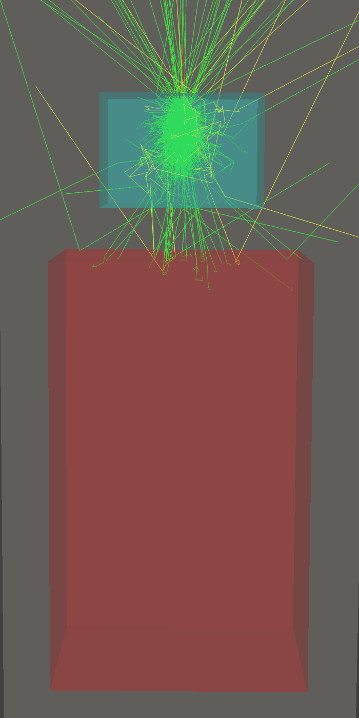 50 GeV e-
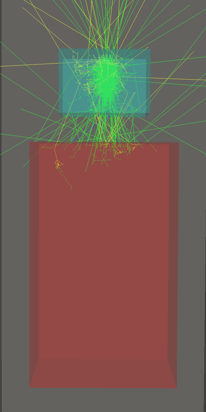 50 GeV y
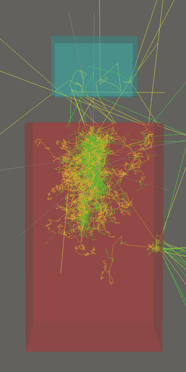 50 GeV K+
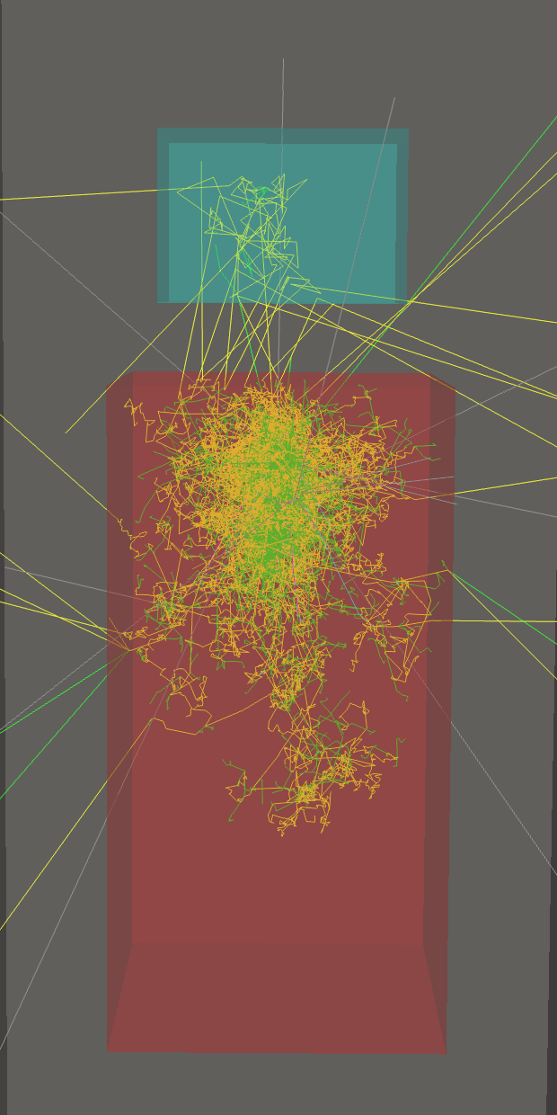 50 GeV K0
As it can be seen, this model replicates the ATLAS calorimeter system nicely, since the EM showers from electrons and photons are concentrated in the ECal, while the hadrons pass through the ECal. Then, these hadrons will undergo hadronic showers in the HCal.